2D Periodic Poisson Solver#
Problem: Solve the 2D Poisson equation \(-\Delta u = f\) with periodic boundary conditions on \([0, 2\pi)^2\), where samples are given on a non-Cartesian (warped) grid.
This example follows the FINUFFT tutorial. It demonstrates how NUFFT enables spectral methods on arbitrary point distributions.
Setup#
First, install nufftax if running on Colab:
# Uncomment the following lines to install nufftax on Colab
# !pip install uv
# !uv pip install nufftax --system
import jax


jax.config.update("jax_enable_x64", True)  # Required for high precision

import jax.numpy as jnp
import matplotlib.pyplot as plt
import numpy as np

from nufftax import nufft2d1, nufft2d2


np.seterr(divide="ignore")
{'divide': 'warn', 'over': 'warn', 'under': 'ignore', 'invalid': 'warn'}
Mathematical Background#
The spectral method for Poisson’s equation has three steps:
Compute Fourier coefficients: \(\hat{f}(k) = \int f(x) e^{i k \cdot x} dx\)
Divide by \(|k|^2\): \(\hat{u}(k) = \hat{f}(k) / |k|^2\)
Evaluate solution: \(u(x) = \sum_k \hat{u}(k) e^{-i k \cdot x}\)
On uniform grids, steps 1 and 3 use FFT. On non-Cartesian grids, we replace them with NUFFT.
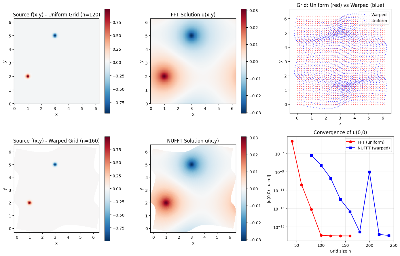
Define the Problem#
We use a source function with two Gaussian bumps and a smooth coordinate transformation.
# Source: two Gaussian bumps
w0 = 0.1
src = lambda x, y: (
    np.exp(-0.5 * ((x - 1) ** 2 + (y - 2) ** 2) / w0**2) - np.exp(-0.5 * ((x - 3) ** 2 + (y - 5) ** 2) / w0**2)
)

# Smooth coordinate transformation: (t,s) -> (x,y)
deform = lambda t, s: np.stack(
    [t + 0.5 * np.sin(t) + 0.2 * np.sin(2 * s), s + 0.3 * np.sin(2 * s) + 0.3 * np.sin(s - t)]
)

# Jacobian matrix for quadrature weights
deformJ = lambda t, s: np.stack(
    [
        np.stack([1 + 0.5 * np.cos(t), 0.4 * np.cos(2 * s)], axis=-1),
        np.stack([-0.3 * np.cos(s - t), 1 + 0.6 * np.cos(2 * s) + 0.3 * np.cos(s - t)], axis=-1),
    ],
    axis=-1,
)
FFT Solver (Reference)#
First, let’s implement the FFT-based solver on a uniform grid as reference.
def solve_fft(n):
    """FFT-based Poisson solver on uniform grid."""
    x = 2 * np.pi * np.arange(n) / n
    xx, yy = np.meshgrid(x, x)
    f = src(xx, yy)

    # Forward FFT
    fhat = np.fft.ifft2(f)

    # Frequency grid
    k = np.fft.fftfreq(n) * n
    kx, ky = np.meshgrid(k, k)

    # Inverse Laplacian filter (zero at k=0 and Nyquist)
    kfilter = 1.0 / (kx**2 + ky**2)
    kfilter[0, 0] = 0
    kfilter[n // 2, :] = 0
    kfilter[:, n // 2] = 0

    # Inverse FFT
    u = np.fft.fft2(kfilter * fhat).real
    return u, xx, yy, f
print("FFT-based solver on uniform grid:")
print("-" * 40)
for n in [40, 60, 80, 100, 120]:
    u, _, _, _ = solve_fft(n)
    print(f"n={n}:  u(0,0) = {u[0, 0]:.15e}")
FFT-based solver on uniform grid:
----------------------------------------
n=40:  u(0,0) = 1.551906153625020e-03
n=60:  u(0,0) = 1.549852227637310e-03
n=80:  u(0,0) = 1.549852190998225e-03
n=100:  u(0,0) = 1.549852191075838e-03
n=120:  u(0,0) = 1.549852191075829e-03
NUFFT Solver#
Now let’s implement the NUFFT-based solver that works on warped grids.
def solve_nufft(n, tol=1e-12):
    """Solve -Δu = f on warped grid using NUFFT."""
    # Parameter grid
    t = 2 * np.pi * np.arange(n) / n
    tt, ss = np.meshgrid(t, t)

    # Physical coordinates (warped)
    xxx = deform(tt, ss)
    xx, yy = xxx[0], xxx[1]

    # Jacobian determinant for quadrature weights
    J = deformJ(tt.T, ss.T)
    detJ = np.linalg.det(J).T
    ww = detJ / n**2  # Quadrature weight = |det(J)| * (2π/n)²

    f = src(xx, yy)
    Nk = int(2 * np.ceil(0.5 * n / 2))  # Number of modes

    # Type-1 NUFFT: compute Fourier coefficients
    fhat = np.array(
        nufft2d1(
            jnp.array(xx.ravel()),
            jnp.array(yy.ravel()),
            jnp.array((f * ww).ravel().astype(np.complex128)),
            n_modes=(Nk, Nk),
            isign=1,
            eps=tol,
        )
    )

    # Convert centered output to FFT ordering
    fhat_fft = np.fft.ifftshift(fhat)

    # Inverse Laplacian filter (zero at k=0 and Nyquist)
    k = np.fft.fftfreq(Nk) * Nk
    kx, ky = np.meshgrid(k, k)
    kfilter = 1.0 / (kx**2 + ky**2)
    kfilter[0, 0] = 0
    kfilter[Nk // 2, :] = 0
    kfilter[:, Nk // 2] = 0

    # Convert back to centered ordering for Type-2
    uhat = np.fft.fftshift(kfilter * fhat_fft)

    # Type-2 NUFFT: evaluate solution at warped points
    u = np.array(
        nufft2d2(jnp.array(xx.ravel()), jnp.array(yy.ravel()), jnp.array(uhat), isign=-1, eps=tol)
    ).real.reshape((n, n))

    return u, xx, yy, f
print("NUFFT-based solver on warped grid:")
print("-" * 40)
for n in [80, 120, 160, 200, 240]:
    u, _, _, _ = solve_nufft(n)
    Nk = int(2 * np.ceil(0.5 * n / 2))
    print(f"n={n}: Nk={Nk}  u(0,0) = {u[0, 0]:.15e}")
NUFFT-based solver on warped grid:
----------------------------------------
n=80: Nk=40 u(0,0) = 1.549915296572036e-03
n=120: Nk=60 u(0,0) = 1.549851996887887e-03
n=160: Nk=80 u(0,0) = 1.549852191030718e-03
n=200: Nk=100 u(0,0) = 1.549851274681522e-03
n=240: Nk=120 u(0,0) = 1.549852191075837e-03
Visualization#
Let’s visualize the source function, solution, and convergence.
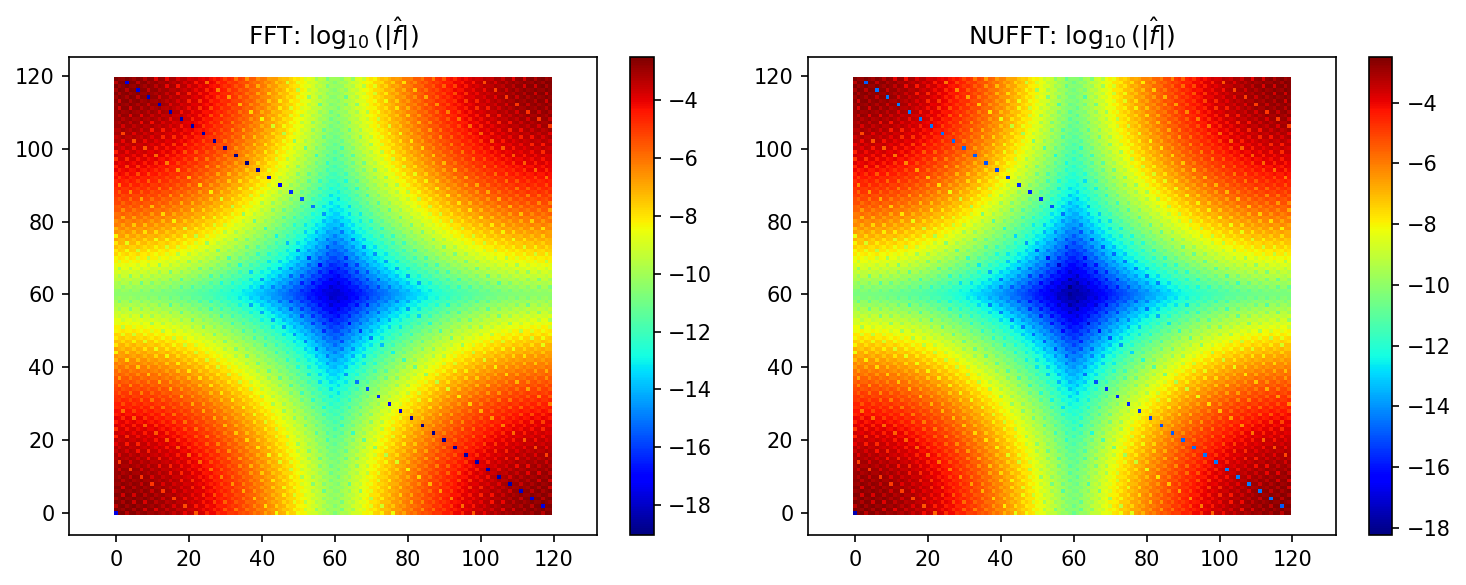
Fourier Mode Decay#
The decay of the Fourier modes \(\hat{f}\) on a log plot for both FFT and NUFFT versions: