MRI Reconstruction from Non-Cartesian Samples#
Problem: MRI scanners often acquire data along non-Cartesian trajectories (radial, spiral) for faster scanning or motion robustness. You need to reconstruct the image.
The forward model (image → k-space samples) uses Type 2 NUFFT, and the adjoint (k-space → image) uses Type 1 with density compensation.
Setup#
First, install nufftax if running on Colab:
# Uncomment the following lines to install nufftax on Colab
# !pip install uv
# !uv pip install nufftax --system
import jax.numpy as jnp
import matplotlib.pyplot as plt
import numpy as np

from nufftax import nufft2d1, nufft2d2
Mathematical Background#
Forward model (image → k-space samples) uses Type 2:
\[y[j] = \frac{1}{\text{norm}} \sum_k x_k \cdot e^{i (k_x[j] \cdot r_k + k_y[j] \cdot c_k)}\]
Adjoint (k-space → image) uses Type 1 with density compensation.
Define MRI Operators#
# Normalization factor (following standard convention)
def compute_norm_factor(shape):
    return np.sqrt(np.prod(shape) * 4)  # sqrt(H*W*2^ndim) for 2D


# Density compensation for radial trajectories
def compute_radial_dcf(kx, ky):
    rho = jnp.sqrt(kx**2 + ky**2)
    weights = jnp.maximum(rho, 1e-6)
    return weights / weights.mean()


# Generate radial trajectory (spokes through k-space center)
def generate_radial_trajectory(num_spokes, num_samples, in_out=True):
    angles = jnp.arange(num_spokes) * (jnp.pi / num_spokes)
    segment = jnp.linspace(-1, 1, num_samples) if in_out else jnp.linspace(0, 1, num_samples)
    radius = jnp.pi * segment
    kx = jnp.outer(jnp.cos(angles), radius).ravel()
    ky = jnp.outer(jnp.sin(angles), radius).ravel()
    return kx, ky


# Forward model: image -> k-space (Type 2)
def forward(img, kx, ky, norm):
    return nufft2d2(kx, ky, img, eps=1e-6) / norm


# Adjoint model: k-space -> image (Type 1 with DCF)
def adjoint(kspace, kx, ky, shape, norm):
    dcf = compute_radial_dcf(kx, ky)
    return nufft2d1(kx, ky, kspace * dcf, n_modes=shape, eps=1e-6) / norm
Load Brain MRI Image#
# Load real brain MRI image
# For Colab, you can download from the repo:
# !wget https://raw.githubusercontent.com/geoffroyO/nufftax/main/docs/_static/brain_mri.npy

try:
    phantom = jnp.array(np.load("../_static/brain_mri.npy"), dtype=jnp.complex64)
except FileNotFoundError:
    # Fallback: create synthetic phantom if file not found
    def create_shepp_logan_phantom(size):
        img = np.zeros((size, size), dtype=np.float32)
        y, x = np.ogrid[-size // 2 : size // 2, -size // 2 : size // 2]
        mask = (x / 0.69 / size * 2) ** 2 + (y / 0.92 / size * 2) ** 2 < 1
        img[mask] = 1.0
        mask = (x / 0.6 / size * 2) ** 2 + (y / 0.8 / size * 2) ** 2 < 1
        img[mask] = 0.8
        mask = ((x + 0.22 * size) / 0.11 / size * 2) ** 2 + (y / 0.31 / size * 2) ** 2 < 1
        img[mask] = 0.2
        return img

    phantom = jnp.array(create_shepp_logan_phantom(320), dtype=jnp.complex64)

img_shape = phantom.shape
print(f"Image shape: {img_shape}")
Image shape: (320, 320)
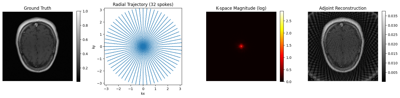
Simulate MRI Acquisition and Reconstruction#
# Generate radial trajectory
num_spokes = 32
num_samples = img_shape[0]
kx, ky = generate_radial_trajectory(num_spokes, num_samples)
norm = compute_norm_factor(img_shape)

print(f"Number of k-space samples: {len(kx)}")
print(f"Normalization factor: {norm:.2f}")

# Forward: acquire k-space data
kspace = forward(phantom, kx, ky, norm)

# Adjoint: reconstruct image
recon = adjoint(kspace, kx, ky, img_shape, norm)
Number of k-space samples: 10240
Normalization factor: 640.00
Visualization#